
Custom Search
The
interwar period in Britain saw a very strong downturn in the level of economic
activity resulting in a very high unemployment peaking 22% in 1920-21. The
unemployment was high compared to both the previous history and the other
countries, although other countries were having problems as well. Furthermore,
the change in unemployment was not just a cyclical movement, the unemployment
level after 1921 recession did not fall to a historical trend level, but remained
permanently higher resulting in an "output gap". This must mean that
the British economy was not going through just a cycle, there must have been
some kind of shocks present to cause a permanent change. In this essay I am
going to discuss the two types of shocks that could have been present: the
demand and supply side shocks.
However
before I start exploring the shocks I must first stress the periodical nature
of unemployment in the interwar era. The two major recessions were in 1920-21
and 1928-32, so the years chose for comparison take account approximately half
of both cycles, which is fair. However one must still note that substantially
different average unemployment rates are obtained for 1920-32 average or
1922-28 average. There are also specific reasons for both of the peaks. I will
not go into them in great detail - I will only look at changes that could have
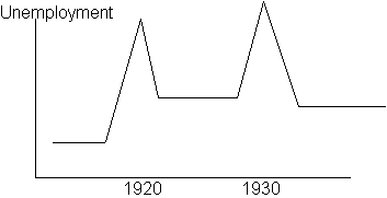
had permanent effect. Unemployment in the interwar era showed a pattern like
this:
Initially
it was argued that supply side shocks caused the peaks in unemployment. Main
concern here has been the strength of trade unions after the war. They managed
to reduce the number of hours worked substantially, without reducing the wage
level, because rather keeping the hourly wage constant employers kept weekly
rate. This amounted to approximately 30% real wage increase. It has been
calculated that the elasticity between employment and real wage is
approximately -3/4. Economy was not experiencing an increase in the
productivity at that time, so this was a serious rise in wage costs for the
firms. This caused the wage gap to rise (Broadberry). The wage gap is the
difference between wage costs and output. This gap only eroded
after second world war.
The
prices were also falling, because of the return to gold. Nominal wages did
adjust, but with a lag and meanwhile people had too high wage. Also workers had
to reduce consumption during first world war that caused high accumulated
savings. They shifted out the budget constraint. People could afford to consume
more goods and more leisure at the same time and thus reduced the hours worked.
However
Dimsdale (1984) showed that the real wage movements were small at that time and
could not account for any major changes. It should be noted that the real wages
were measured by RPI by Broadberry. GDP deflator should have been used instead
to get the rise in the producer wage cost. This change will eliminate long term
effects of the gap, by 1922 there is no gap anymore. Also the calculation was
for all people, the wage was increased only by 18% for the heads of households
in full employment.
In
long term, however the initial high employment had permanent effects as
explained by the hysteris theory. This will mean that as the number of
unemployed rises, the number of long-term unemployed rises as well. They will
lose the hope of getting a job and will give up trying. They will also have low
probability of being re-employed, as employers like recent practice.
Insider-outsider theories explain the persistence as well, as the
institutionalised wage setting covered 3/4 of the working population.
Outsiders, that were unemployed, could not affect the wage level and thus the
wage level did not come down when unemployment rose. Unions were also using
wage relativities to determine their demands (wanted to have as much as other)
and had co-ordination failures. This meant no union wanted to be the first to
give in and reduce the wage level first.
There
is however not much empirical evidence for long-term unemployment. There was a
group of people who had very high turnover in unemployment, that means they
were changing jobs very often. High turnover meant less job security and lower
pay. It can be explained by the change in the benefits level.
Benefits
were increased after 1921 and they were made available to more people. People
could now take some time off between looking for new jobs. They were also given
unemployment benefit from the first day they became unemployed, so firms were
using the benefits for supporting the wage - they employed people for short
times, made them redundant and then re-employed. Maki and Spindler(1979) have
found 3 ways in which an increase in the benefit level can cause unemployment.
First, more people will register themselves as the labour force to claim
benefits. This happened with women registering more during the interwar period.
Secondly the effective supply of labour decreases due to increase in searching
time and finally demand for labour will decrease as firms are more willing to
lay off workers or put them to part time work.
Crafts
found little evidence of benefits affecting the employment, though.
Unemployment Assistance Board showed the hopelessness of long term unemployment
and argued that it was unlikely to be voluntary. In 1936 73% of unemployed
lived below the poverty line, so they are unlikely to receive too many
benefits. And according to national statistics, only about 150 000 workers were
in some kind of work sharing system, so the cheating of the system was likely
to be insignificant. However Benjamin and Kochin (1979) have found evidence to
support that the unemployment was caused by the increase in the replacement
ratio (what percentage a person can earn of their wage when they are on
benefit). However calculations of this replacement ratio are rendered less
valid again when we use data for the heads of households alone not for a man
with a wife and two children (as Benjamin and Kochin did). Eichengreen first
looked some household evidence in the New Survey of London Life and Labour
(1928). This showed that the heads of families never chose the unemployment,
although some secondary workers did.
The
replacement ratio rose only after 1922, when new Acts were passed, but
significant employment existed already in 1920-21. Benjamin and Kochin could
also give no explanation for the difference in unemployment levels between
different industries. Matthews have argued that the real benefit level, not the
replacement ratio, caused unemployment. This view arises from the fact that as
the prices fell the value of real benefits rose over the period. and so did
unemployment. But the wages actually
fell in line with prices - if people would have become voluntarily unemployed,
then the employers would have bid up the wage level to attract them back, but
they clearly did not.
Smyth
has done a major criticism to Benjamin and Kochin. He said they used an
inappropriate ad hoc model. Benefit basically affects supply, but its effect is
lost GDP, which is demand. The government could also not alter the benefit to
wages ratio, it could only determine the absolute level of benefits. So
absolute benefits and not the ratio should be used.
Huton found no evidence of more search for
employment. "The behaviour of the unemployed in searching for employment
gives no evidence that the possibility of drawing unemployment insurance
benefit has retarded the efforts of the unemployed to get back to work. It has
removed the cutting edge that would otherwise attend that search"(Wright).
The models of unemployment are also not robust. Worswick showed that if one
takes out the recession year 1920, then the result will not hold.
Changes
in the age/sex ratio and arising due to the natural increase in unemployment
were also permanently affecting unemployment. Especially as older people, once
made redundant, were far less likely to get a new job. And the population got
older. But these effects were relatively small. Still, women and young people
were less likely to be unemployed, and higher social class meant less
unemployment too. Unemployment was initially high in these industries that were
expanded during the War, but later unemployment rose in coal also and in other
staple exports industries. Industries towards home markets have less
unemployment. Unemployment is also regional, it was very high in North and
West, in some places even 70%. These
facts led people
to think the unemployment occurred due to structural change to newer industries
from the old staple ones.
It
was estimated that 25-45% of the unemployment was structural. Alcraft -
Richardson took and optimistic view and said that the resources were
transferred to new industries. But there is not much evidence for this
according to Mathew-Smee. They noted that the output growth was not very high
in new industries. Total factor productivity was also not changing much. In new
industries TFP should be rising fast. It was also noted that there was a
greater change during the actual War period than during the interwar. New
industries were also less capital intensive, so employment should have risen.
Writers found no correlation between mergers and efficiency gains, too. So the
structural change should not be taken as an explanation.
As
seen from this widely scattered evidence on supply side, there were shocks
present, but none of them was very big and many did not affect the output
permanently. I now turn to look at the demand side shocks. Frequently demand
side shocks are not permanent and thus tend to be overlooked. However, recent
historians have shown there were permanent demand shocks present during the
interwar era.
Main concern has been on the return of the
Britain to the gold standard with the pre-war parity. There is some strong
comparative evidence supporting this. Scandinavian and British countries used fast
transition to gold standard. France, Belgium return to gold at a depreciated
rate (over 20 years). Rest of the Europe was not concerned about the
transition, they had other problems from the War to sort out (Germany). Britain
goes to restrictive monetary policy and sticks with it. France had restrictive
policy but it defeated that as soon as problems arose. And evidently,
Scandinavia and Britain face the biggest recession, it is mild in France and
almost non-existent in Germany.
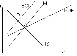
Flexible
exchange rates and restrictive interest rates caused deflationary expectations
and decreased exports. This graph shows an equilibrium A with a given exchange
rate. If exchange rates rose with interest rate increase appreciation of an
exchange rate to B will happen:
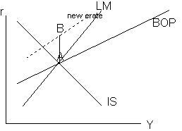
The
actual appreciation was much bigger than we expect, because of the overshooting
of the monetary theory. Different markets have different adjustment rates.
Assets markets are quick, but goods markets have a number of rigidities, so
they adjust slowly. If the government made the announcement (1919) of
restrictive policy, a quick adjustment to B happened:
So
initially the exchange and interest overshot and then adjust slowly downwards
as IS shifts. That is exactly what we observe, there was a big overvaluation in
1919-21. Overshooting has been observed also in other countries with flexible
exchange rates. Overshooting leads to too high exchange rate and contraction of
export that should lead to a fall in GDP. High interest also decreased the
investment and the national income. But for sure it is only the price of
exports and imports that changes, but on the balance of payments account we are
concerned with the value. Value will not decrease if the price increases (for
imports) when the demand for imports is inelastic. In fact it is quite the
opposite. Similarly in order to get a deterioration in the current account we have to assume
elastic exports, but there is no strong empirical evidence for that.
But
the exchange rate change was only temporary. If one wants to explain why the UK
became locked in to the lower GDP level one has to look at the multiplier
effects. Imports are leakages and when they increased, GDP decreased by more
and possibly permanently. However writers have assumed that the high exchange
rate lead to an automatic increase in investment and decrease in exports.
We
are unlikely to find a single explanation for the high unemployment. Perhaps
the overshooting and wage gap together made the UK to
lose its trading
position and competitiveness and changed the whole world trade patterns. Once
the competitors had set in the UK they did not leave when the UK’s industry
made a comeback. Foreign firms might have had high set-up costs, instead of
leaving they lowered their markups. There is some empirical evidence for that,
particularly the rise in import ratios from 20% of GDP before the War to 24%
after.
There
was also lots of optimism and new investment up to 1918. Many debts were taken
out with near 0 real interest rate. As the economy deflated real interest rose and real debt burden shot up. Empirical evidence shows that the
debt to income ratio rose from 1.6 in 1913 to 2.8 in 1920's. In France, for
example, the inflation was eroding some of the debt.
It is
thought at present that the combinations of both supply and demand
side lead to persistence of low GDP and high unemployment during the interwar
period. Although supply side reasons tend to be weaker, there are many of them
and they most probably reinforced the big demand shock of
returning to the
gold standard.